The Model Statistics page provides clarity and information about machine learning models, specifically aimed at making the complex world of models more understandable, even for non-technical users. After every model training session, various statistics and graphs become available to help users interpret the model’s behavior and predictions.Currently, this functionality is available for Churn and Response Prediction models.
The second part of this page is dedicated to model explainability using SHAP (SHapley Additive exPlanations) values. SHAP values provide insight into how the model makes predictions by attributing the importance of each feature.
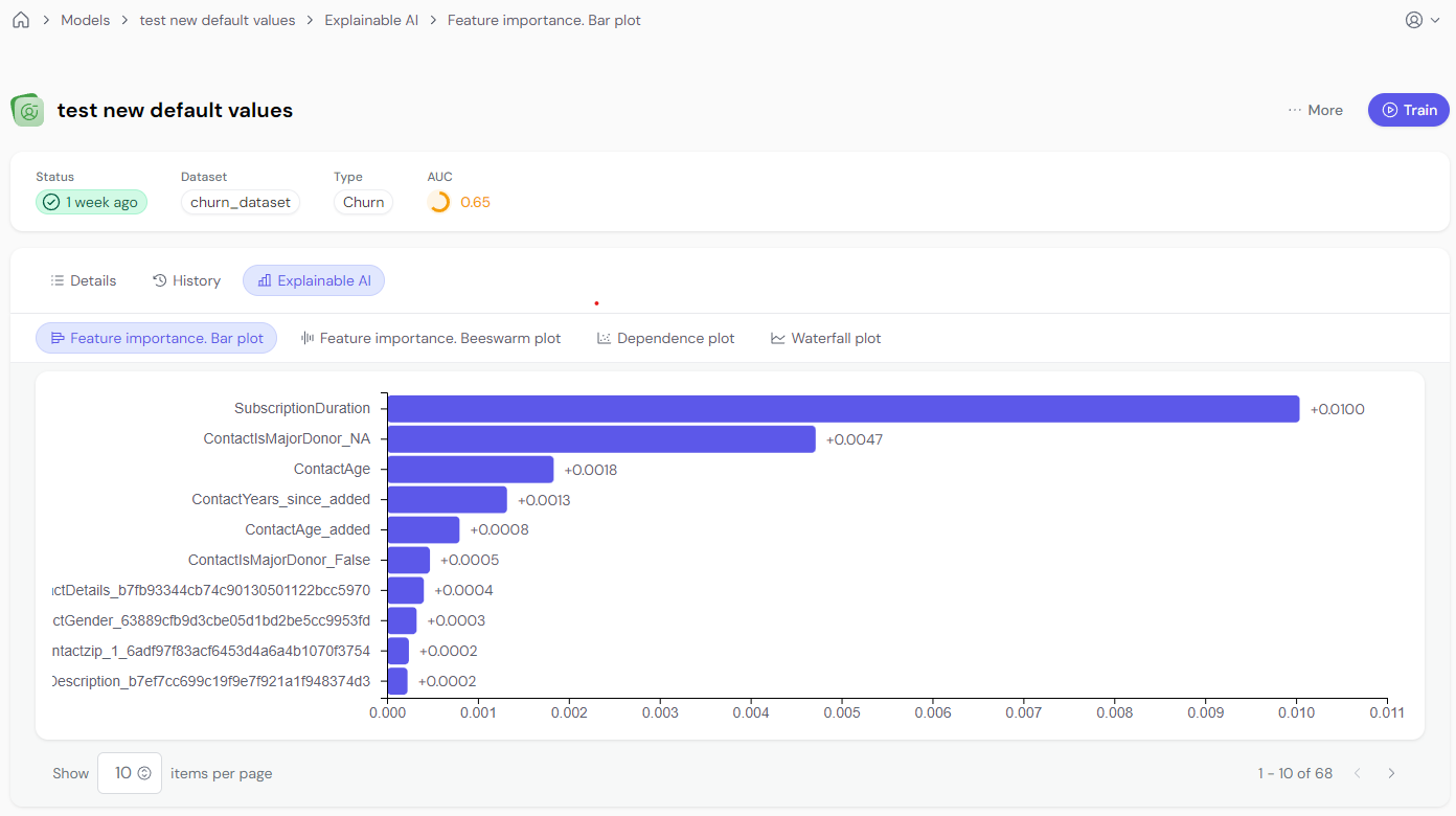
A bar plot displays the global importance of each feature, indicating which features the model used most to make predictions. The size of the bar reflects the importance, but remember: larger bars don’t mean larger SHAP values—it just means those features were important to the model.
This plot shows which features the model considers important, helping users understand the most influential factors. Remember, higher bars mean higher importance, not necessarily higher SHAP values.
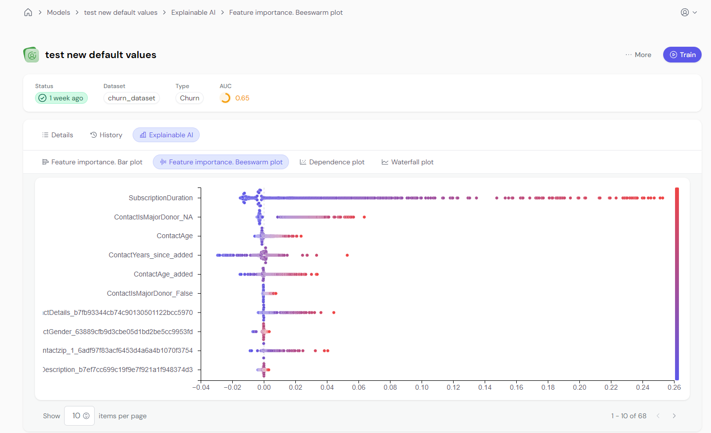
The beeswarm plot provides a global view of feature impact, displaying individual SHAP values for all rows in the training dataset. The color represents the feature’s value (high/low), and the x-axis represents the SHAP value (positive/negative impact on the prediction).
Left-right on the x-axis shows the SHAP value, representing the feature’s impact (positive or negative) on predictions.
Top-bottom shows features ranked by importance.
Color coding: Red means high feature values, blue means low feature values.
Each point represents a row in the training data, with the color showing whether the feature’s value was high (red) or low (blue). Points on the right have a positive impact on predictions, while points on the left have a negative impact.
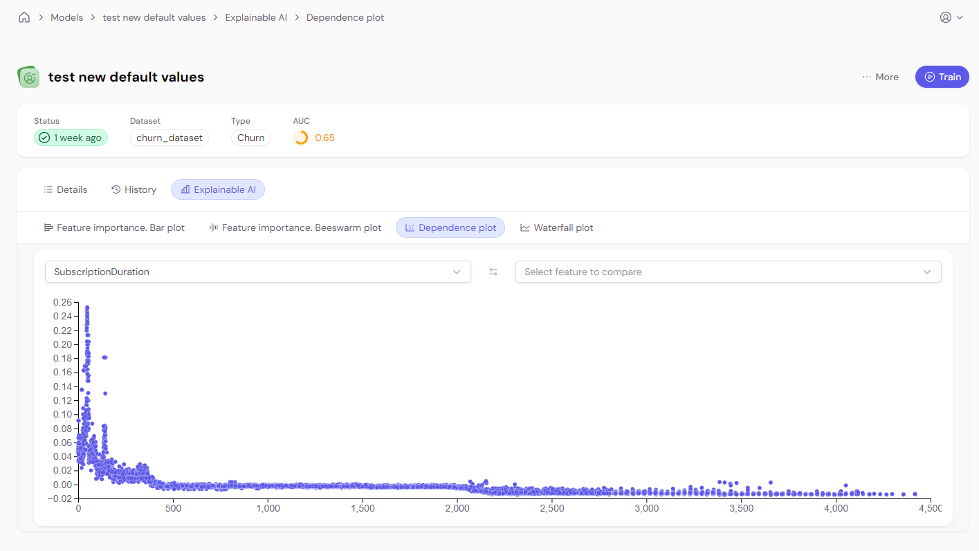
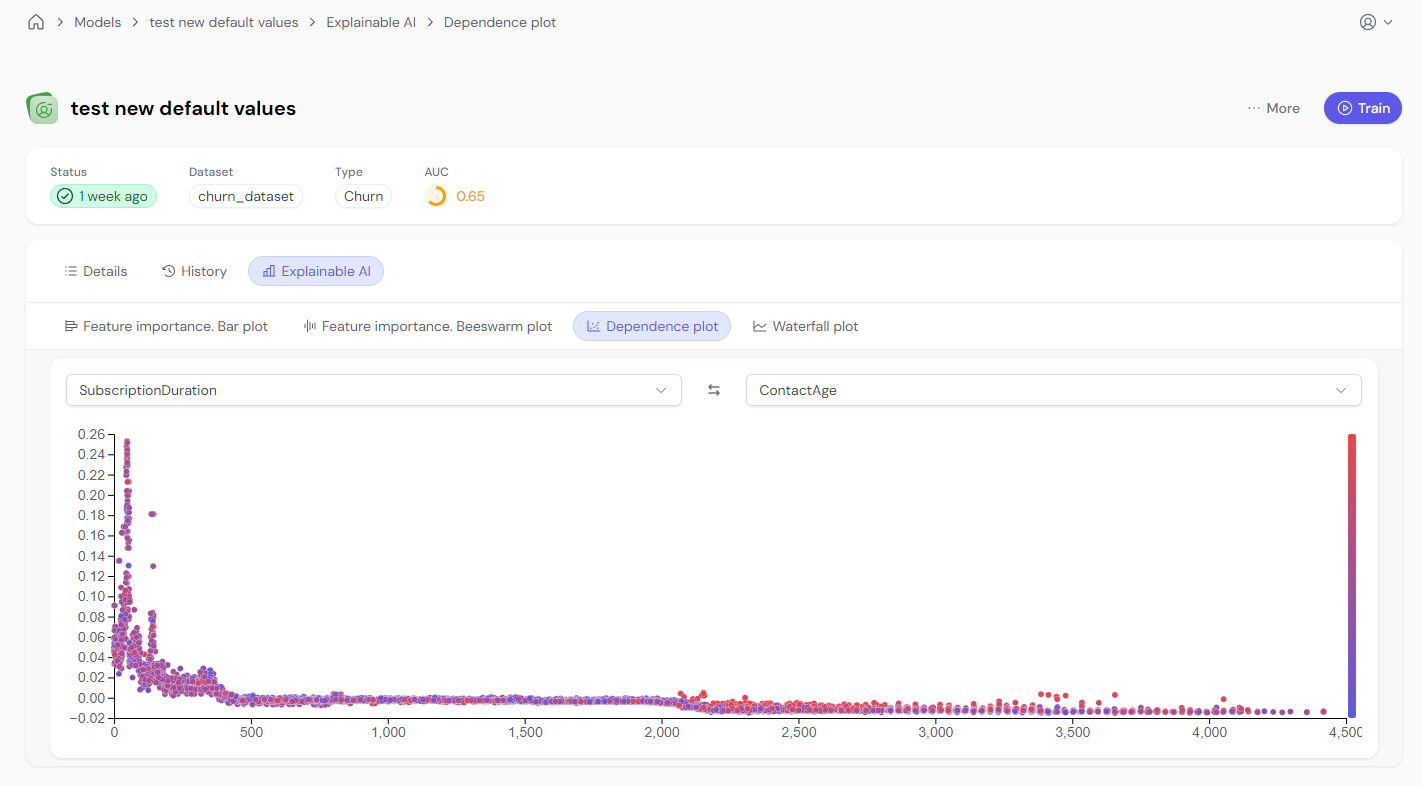
Dependence plots allow users to visualize how a feature impacts the model’s predictions. You can view these plots with one feature or two features for more detailed analysis.
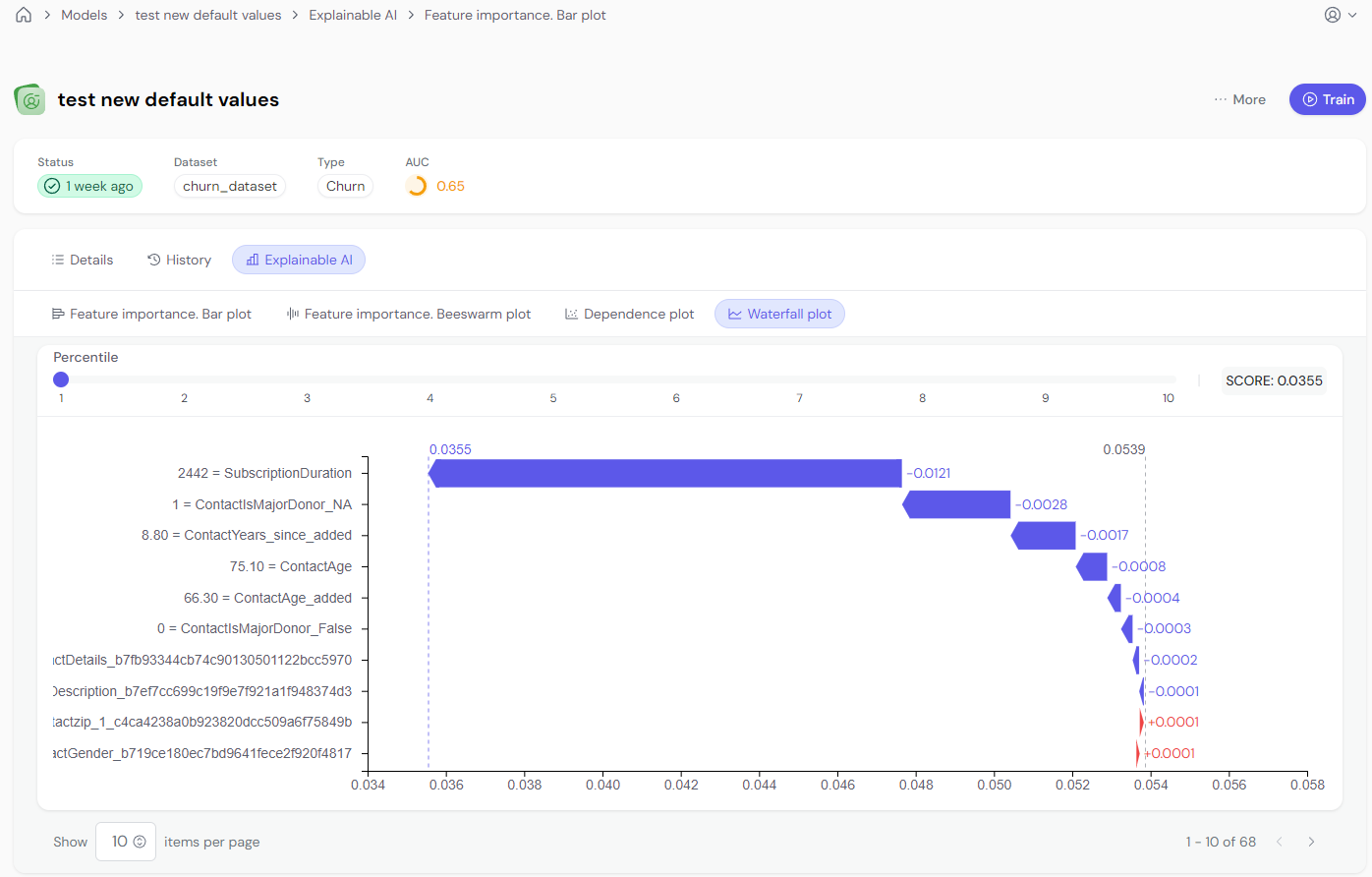
The waterfall plot breaks down the model’s prediction for a specific row, showing how each feature contributes to the final score. This is an excellent way to understand how the model arrived at a specific decision.
The top right corner displays the predicted score.
A slider allows you to navigate between different rows of data (10 rows available).
Waterfall plots explain the prediction for a specific row. Each feature either increases or decreases the score. You can select up to 10 rows using the slider.
The first section provides key performance metrics for each model after training. The most important metrics include:
AUC-ROC (Area Under the Receiver Operating Characteristic Curve): Measures the model’s ability to distinguish between classes. A higher value indicates better performance.
AUC-PR (Area Under the Precision-Recall Curve): Focuses on how well the model performs when dealing with imbalanced datasets. It shows precision (positive predictive value) vs. recall (true positive rate).
Use cards to display these metrics clearly, perhaps side-by-side to let users compare:
AUC-ROC
Area Under the Receiver Operating Characteristic Curve. Indicates how well the model distinguishes between classes.
AUC-PR
Area Under the Precision-Recall Curve. Measures performance with imbalanced data.
The Model Statistics page provides crucial insights into machine learning models through performance metrics and SHAP-based explainability tools.
By using visual aids like bar plots, beeswarm plots, dependence plots, and waterfall plots, users can gain a deeper understanding of how the model works and which features drive the predictions.
These tools empower non-technical users to interpret and trust machine learning models.